Uncertainty based capacity planning

The active use of risk management is permeating more and more business activities. To geeks like myself, this evolution appears somewhat slow – but that just leaves opportunities for those who lead the change to gain significant competitive advantages over those who hold on to former approaches.

I have a background in manufacturing capacity planning – and when I did that decades ago, it was firmly based on single-point estimates:

• · Sales of product “A” was 150.000 in January, i.e. it could neither be 149.000, nor 170.000
• · Capacity requirement on equipment “X” was 24 hours/100 pieces, i.e. neither 22 nor 25 hours
• · Hence, capacity need for January for product “A” on equipment “X” was exactly 3.600 hours
• · We aim to have a 90% utilization of equipment “X”, and hence, we build capacity to be 4.000 hours

Based on that, we expected to be able to deliver what is needed.

However, we knew, that there were – potentially – significant uncertainties embedded in the assumptions on sales and capacity requirements and hence – we could not be certain we would be able to meet the actual need when that materialized. And true enough, we did experience several instances of shortcomings (more than 10%).

Today, by leveraging Monte Carlo simulation (MCS), we can enhance the value of the capacity planning, and plan to e.g. ensure a 90% delivery service despite the uncertainties of the assumed data. In this article I use @Risk from Palisade, but could just as easily have used ModelRisk from Vose – both of which are add-on tools to Excel.

Target first … the aim of capacity planning is to ensure the capability of meeting demand with a defined certainty (delivery service) – without costly overinvesting in equipment and/or inventory.

 

Demand uncertainties

Forecasts are made in terms of single point estimates whereby we forecast one explicit demand for each product for each month, or whatever period we use. Intuitively we know this is not valid – but we need to analyse the level of validity to get any further. Fortunately, the validity of these forecasts is easily analysed by looking at the variation between past forecasts and actual values.

Create a table of forecasts and actual values, and calculate a factor by simply dividing the actual value by the forecast (i.e. an A/F factor). If/when the value is above 1, actual sales exceeds the forecast, and if/when the factor is below 1, actual sales is below forecast.

When looking at these numbers be aware of the mathematics embedded. If actual is four times the forecast, the factor becomes 4,0. If actual is a quarter of the forecast, the factor becomes 0,25. Hence, the factors inherently becomes right skewed. Then again – being asked to deliver 4 times the forecasted value is most likely more problematic than having 75% of production not being sold. Both @Risk and ModelRisk provides tools to analyse a dataset of A/F factors.

To add to the accuracy, it may be highly valuable to graph these and look for systematic “errors” or variations, e.g.:

• · Driven by seasonality (e.g. we tends to under-forecast summer demand and over-forecast winter demand).
• · A low A/F factor in one month tend to lead to a high – or a low – factor in the subsequent month. Simple correlation analyses of a dataset will show this.
• · The volatility of product A may be highly correlated (positively or negatively) with the volatility of product C. Excel itself provides the possibility to detect such correlations.

Graphic displays and data analyses of these factors can provide strong indications of systematic errors. It will be easy to systematically model all found correlations despite the value of the correlation factor. However, I do not recommend using this if/when correlation factors are below 0,7 as the validity of these may be coincidentally based on your analysed data and they will not affect the outcome significantly anyway.

When addressing such errors, I have been in touch with companies, where demand volatility on some product lines were as high as +/- 50%, and where cross product line correlations were more than 0,9 and hence very impactful in the modelling and capacity demand.

Some companies do capacity planning based on product demands of each single product, others (I assume, most) will do this based on product groups/product lines where a range of products are reasonably similar and where demand for one product tend to follow the average of this product line, and hence create an adequately stable average.

Such variations are easily modelled in a MCS model, e.g. like the below modelling:

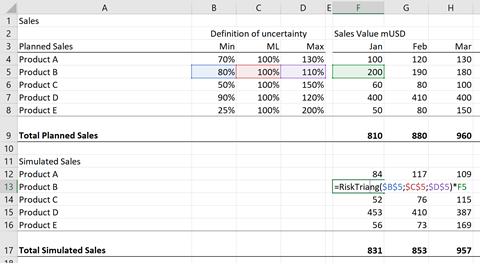
For the highlighted product B, we have analysed that a forecast of 100 will lead to an actual demand of somewhere between 80 and 110 – not very dramatic. For product C the volatility is +/- 50% for each monthly forecast.

Leveraging these uncertainties, the sales of each iteration is calculated, here using a triangular distribution. This is done for each product/product line for each month., and hence we calculate a demand profile for each month on product (/line) as well as total level.

In some cases, demand of product A is correlated with the demand of e.g. product D – which can be embedded in the modelling as well. Both @Risk and ModelRisk have easy ways of doing this.

Capacity uncertainties

If/when capacity planning is done using data for individual products, the amount of data used will be quite significant as companies may have a product portfolio of several hundred products. To simplify, most companies opt to plan on product line level, whereby the needed planning is reduced to perhaps 20 or 50 product lines.

The downside of doing this is, that the equipment requirement needed to produce e.g. 1 mio USD worth of a given product line product will differ depending on the actual mix of products demanded. However, my experience indicates, that the demand mix of products within a product line tend to be somewhat stable, and hence have little (but not ignorable) uncertainties.

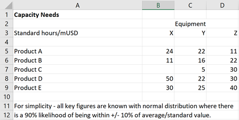
The modelling can look like this table, where:

• · One mio USD worth of product line A will require 24 hours on equipment X and 22 hours on equipment Y plus 11 hours on equipment Z.
• · Product (line) C is shown not to rely on equipment X etc.

The volatility of these data are often easily analysed using manufacturing data the company already have, and which planners are well accustomed to address.

For this article, I have opted (incorrectly in real life) to use one and the same level of uncertainty on all such capacity key figures.

Modelling capacity needs

Combining the two above sets of input, we can now model the capacity planning, which is done for 5 product lines A … E on three pieces of equipment X … Z.

By doing this modelling, we do not only get the capacity need based on the average demand, which for capacity planning often is rather irrelevant. Assuming the company has committed or targeted a 90% delivery service, we can directly simulate and find the capacity needed to be 90% certain actual demand can be met.

Normally, and based on the traditional use of single point estimates, companies seek to ensure delivery service by setting limits on planned capacity utilization and/or embed volatilities in inventory profiles. My perspective is, that both of these approaches, as well as combining these, are based on “gut feeling” and non-measured experience – and hence, that the described leverage of MCS can provide more valid and more precise data – allowing tighter capacity investment and inventory value control without jeopardizing meeting the targeted delivery service.

 

Calculating simulated equipment demand

As stated by combining the input on sales and key figures, we can now calculate the capacity need when taking data uncertainties into due account.

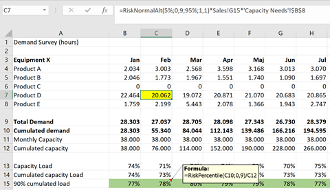
In the highlighted cell (C7), the capacity demand for product line “D” on equipment “X” in February is calculated based on the normal distribution (on the capacity key figure) multiplied with the simulated sales and the capacity key figure, which in this iteration leads to 20.062 hours.

This is not different from all other capacity calculations – what IS different is the ability to calculate the shown line 15, where we show the cumulated capacity load at the 90^th percentile, i.e. the capacity load will be 90% certain to be under.

The cumulated capacity load is used, as the capacity requirement of any individual month may exceed 100%, but can be handled by producing for inventory in earlier months where demand is lower – and hence, avoid require equipment investments.

The insight of what is the 90% peak demand with the demand and key figure uncertainties taken into account is not available when using traditional single point estimate planning. The value of the approach comes from acquiring this insight with even a relatively simple model.

Based on the case example, the MCS approach can show the difference between what is being planned using a traditional approach, and what is needed to meet delivery targets.

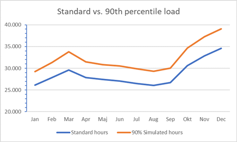
For the example model, this is the hours needed on equipment X over the year.

The blue line shows the outcome of the standard approach, where each month shows a need below 35.000 hours.

The orange line, which is based on a simulated 90^th percentile need shows a higher level in general, and December actually exceeds the modelled 38.000 hours of capacity, which add the need to “over produce” on November to build inventory that can be drawn upon to cover December demand without investing in new equipment.

For real life use, the model can be further tailored and qualified by adding e.g. operational risks like equipment breakdowns, slowdowns or the like as well as any other uncertainties pertaining to the relevant capacity planning.

Leveraging this MCS based approach will help companies to:

• · Invest in additional equipment when needed to meet the 90% delivery service target – without investing too soon “just in case”
• · Build and leverage optimal inventory levels – whilst meeting the delivery service commitment

And thereby enhance the economic value added by operations.

Closing

This MCS based approach to capacity planning is not risk management as such. However, it is my experience, that risk managers are more inclined and experienced in working systematically with uncertainties – and know how to use Monte Carlo simulation (or should). Hence, deploying an MCS based planning approach is an opportunity for the risk manager to add value to the company.

If you find this article interesting, and wish to see the underlying example model, send me an email on hl@aktus.dk, and I will send you this model. If you use ModelRisk rather than @Risk, I know ModelRisk has a feature, which automatically transforms formulas to ModelRisk formulas, enabling you to use ModelRisk as well.